Kolmogorov-Arnold Networks (KANs) - What's the fuss about?

I was resting after a busy work day some weeks ago when I came across a post about the paper KAN: Kolmogorov–Arnold Networks. The paper was not even published yet and there were already more than 8K stars on its github repository in less than a week. It seems to have taken the internet by storm and that is all anyone on Data Science LinkedIn seemed to be talking about. Could this really be the next big thing for Deep Learning and AI? Are the “Yet another big LLM with an even bigger context length” model releases every other week getting boring? I searched around for simpler but comprehensive explainer articles to digest the paper and couldn’t find one, so I decided to write one.

To help understand KANs, let’s take a quick primer on Multi-layer Perceptrons (MLPs)

MLPs and The Universal Approximation Theorem

At the core of every machine learning algorithm is the desire to estimate functions. Given an input, we want a function that returns a desirable output. From transactions to customer churn predictions, images to cat/dog classification, etc. The problem then is, how do we define such complex functions? In the 80s, researchers discovered that theoretically, any function could be approximated by a neural network to some arbitrary accuracy and this became known as the universal approximation theorem.

The Universal Approximation Theorem states that a neural network with at least one hidden layer of a sufficient number of neurons, and a non-linear activation function can approximate any continuous function to an arbitrary level of accuracy.

To understand this, let’s break it down:

1. Neural Networks as Function Approximators: At their core, neural networks are designed to estimate functions. Given an input x, the network computes an output y through a series of transformations. The goal is to adjust these transformations so that the network accurately maps x to y.
2. Layers and Neurons: A neural network consists of layers of neurons. Each layer applies a linear transformation to the input data, followed by a non-linear activation function.
   Mathematically, for a single hidden layer, this can be expressed as:
   

   $$y = \sigma(W x + b)$$

   
   where \(W\) is a weight matrix, \(b\) is a bias vector, and \(\sigma\) is a non-linear activation function.

3. Activation Functions: This function introduces non-linearity, enabling the network to model complex relationships in the data. The choice of activation function is crucial and common activation functions include the sigmoid, hyperbolic tangent (tanh), and Rectified Linear Unit (ReLU).

UAT Implications and Deep Learning Training

The Universal Approximation Theorem (UAT) underscores the power of neural networks and deep learning. With sufficient layers and neurons, and the right activation functions, these networks can approximate any function, allowing them to solve complex tasks like image recognition, natural language processing, and more.

But here’s the kicker: just having a powerful formula isn’t enough. While we have the formula, we don’t initially know the exact weights and biases needed to make accurate predictions. This is where training comes in.

Training a neural network involves feeding it data and adjusting its parameters (weights and biases) to minimize the error in its predictions. Think of it as teaching a dog new tricks. You start with random behaviour, but with consistent training and a lot of treats (in this case, data and optimization), the dog learns to perform the desired tricks accurately.

Here’s a step-by-step breakdown of the training process as a refresher:

1. Initialization: Start with random weights and biases.
2. Forward Pass: Input data is passed through the network, and predictions are made.
3. Loss Calculation: Measure how far the predictions are from the actual values using a loss function (e.g., Mean Squared Error for regression tasks).
4. Backpropagation: Calculate the gradient of the loss with respect to each weight and bias, essentially determining the direction and magnitude of adjustments needed.
5. Parameter Update: Adjust the weights and biases using an optimization algorithm (like Gradient Descent) to reduce the loss.
6. Repeat: This process is repeated for many iterations (epochs) until the network’s performance stabilizes and the loss is minimized.

So far so good, this is the basis of more complex networks like the Convolutional Neural Networks (CNN) for vision and even the all-powerful Transformers that are the backbones of today’s Large Language Models.

Kolmogorov-Arnold Theorem (KAT)

The Kolmogorov-Arnold Theorem (KAT) takes a different approach to function approximation. It states that any multivariate continuous function can be represented as a superposition of continuous functions of one variable and addition. In simpler terms, this means breaking down a function of several variables into functions of a single variable.

Mathematically, this can be expressed as:

$$f(x_1, x_2, \ldots, x_n) = \sum_{i=1}^{2n+1} \phi_i \left( \sum_{j=1}^{n} \psi_{ij}(x_j) \right)$$

where \(\phi_i\) and \(\psi_{ij}\) are continuous functions of one variable.

The Kolmogorov-Arnold Theorem (KAT) is a powerful theoretical tool, stating that any multivariate continuous function can be decomposed into a sum of continuous functions of a single variable. As the authors noted, the only truly multivariate function in KAT is the sum! However, this decomposition comes with significant limitations, particularly when applied to practical problems in machine learning.

One of the main limitations of KAT is the non-smoothness of the decomposed functions. In practice, the functions \(\phi_i\) and \(\psi_{ij}\) resulting from the KAT decomposition can be highly irregular or non-smooth. This non-smoothness makes these functions difficult to approximate and optimize using standard machine learning techniques. Non-smooth functions can lead to poor convergence rates and instability during training, making the learning process inefficient and less reliable.

In the context of neural networks, smooth activation functions like the sigmoid or ReLU are preferred because they facilitate better gradient flow during backpropagation. Non-smooth functions disrupt this flow, causing vanishing or exploding gradients, which hinder the training process. This issue is particularly pronounced in deeper networks, where the compounded effect of non-smoothness can severely degrade performance.

Moreover, the practical implementation of KAT requires determining suitable \(\phi_i\) and \(\psi_{ij}\) functions for a given problem, which is not straightforward. The theorem provides a theoretical guarantee of existence but does not offer a constructive method to find these functions. As a result, applying KAT in real-world scenarios often involves heuristic methods or additional assumptions, which may not always yield optimal results.

Kolmogorov-Arnold Networks (KANs)

The paper proposes overcoming these limitations by using smooth, trainable functions within the Kolmogorov–Arnold Networks (KAN). By incorporating splines and trainable activation functions, KAN aims to retain the theoretical benefits of KAT while mitigating its practical drawbacks, providing a more efficient and stable approach to function approximation.

KAN leverages the Kolmogorov-Arnold Theorem in a novel way. It structures the neural network to mimic the theorem, effectively creating a 2-layer neural network which can then be expanded to an arbitrary number of layers to achieve a more complex model.

Splines as KAT Functions

In the world of KANs, splines are the secret sauce that makes the magic happen. But what exactly are splines, and why are they so important?

Splines are piecewise polynomial functions used to create smooth and flexible approximations of more complex functions. Think of them as the duct tape of mathematical functions: they can patch together simple polynomial pieces to form a smooth curve. This is particularly useful in KAN because it addresses one of the major limitations of the Kolmogorov-Arnold Theorem (KAT): the non-smoothness of decomposed functions.

The paper delves into how KAN uses splines to improve upon the KAT functions. Here’s a deeper look at how this works:

1. Piecewise Polynomials: Splines are constructed from multiple polynomial segments. Each segment is defined over a specific interval of the input space. This segmentation allows splines to handle local variations in the data more effectively than a single global polynomial.
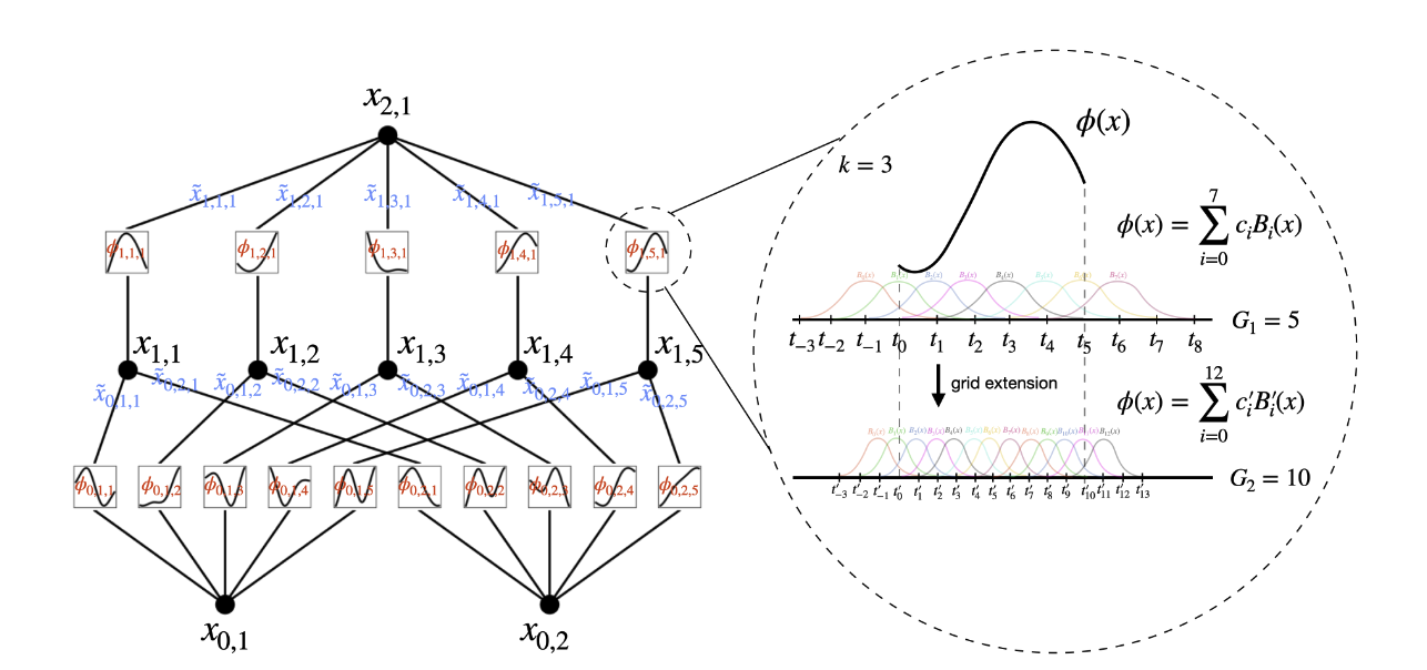
2. Smooth Transitions: The polynomial segments are stitched together in such a way that the transitions between them are smooth. This smoothness is crucial because it ensures that the overall function remains continuous and differentiable. The KAN architecture takes advantage of this by using B-splines, which are a specific type of spline that provides a high degree of smoothness and flexibility.
3. Flexibility and Adaptability: By adjusting the coefficients of the polynomial segments, splines can approximate a wide range of shapes and patterns. This flexibility is what makes them so powerful in function approximation. In the context of KAN, splines are used to model the \(\psi_{ij}\) functions from the KAT formulation. This means that instead of dealing with potentially rough and jagged KAT functions, KAN uses smooth, continuous splines that are easier to optimize and work with. And what’s more? the number of spline segments can be varied to better fit the function.
4. Implementation in KAN: The paper details how KAN implements these splines within the network architecture. Each spline is represented as a linear combination of basis spline functions (B-splines), which are then used to construct the \(\psi_{ij}\) functions. The coefficients of these basis splines are learned during the training process, allowing the network to adaptively fit the data.

Trainable Activation on Edges

KANs introduce a fascinating innovation: trainable activation functions on the edges of the network. In traditional neural networks, activation functions like ReLU, sigmoid, or tanh are fixed functions applied to the outputs of neurons at the multivariate level. These functions help introduce non-linearity into the model, enabling it to learn complex patterns. However, in KAN, the activation functions are not fixed; they are trainable and used at the univariate level, meaning the network can learn the optimal form of these functions during training.

Here’s how KAN achieves this:

1. Custom Activation Functions: Instead of using pre-defined activation functions, KAN uses custom functions that can be adjusted based on the data. These custom functions are parameterized and their parameters are learned during the training process, just like weights and biases.
2. Edge Functions: The term “on the edges” refers to applying these trainable activations between the layers of the network. In graph theory (which neural networks can be viewed through), edges connect nodes (neurons), and in KAN, the activations on these edges are dynamic and can adapt to the data.
3. Learning the Activation Functions: The paper describes using splines (piecewise polynomials) to represent these trainable activations. By learning the coefficients of these splines during training, KAN can tailor the activation functions to better fit the underlying patterns in the data. This flexibility allows KAN to capture more complex relationships than fixed activation functions.

To put it simply, The non-linear part of traditional neural networks is fixed and not trainable. Although there are variations like the Parametric ReLU (PReLU) that allow training, it is still very limited as the parameters are global. KANs on the other hand provide fully trainable local non-linear functions for each input.

Interpretability, Especially for Science

One of the standout features of Kolmogorov–Arnold Networks (KAN) is their interpretability, which is particularly valuable in scientific applications. Traditional deep learning models, while powerful, often act like black boxes. They often make accurate predictions, but understanding how they arrive at those predictions can be challenging. This lack of transparency can be a significant drawback, especially in fields like science and medicine where understanding the reasoning behind a model’s output is crucial.

KAN addresses this issue by structuring the network in a way that makes it easier to interpret. Here’s how:

1. Decomposition into Simpler Functions: KAN leverages the Kolmogorov-Arnold Theorem to decompose complex functions into sums of simpler functions. This decomposition means that the network’s decisions can be traced back to these simpler, more understandable functions, making it easier to see how different inputs contribute to the final output. While MLP functions are also decomposable, much of the learning occurs at the multivariate level where activation functions are applied, using only simple linear univariate functions (\(W_ix_i\)). KANs on the other hand learn non-linear B-splines at the univariate level.
2. Symbolic Formula Extraction: The authors claim they made it possible to recover a symbolic representation of the learned function using SymPy. This will help to discover interesting equations in science.
3. Integrating Prior Knowledge: With a knowledge of the problem domain, one can easily design a more fitting KAN. This is often the case in scientific research but not in real-life problems. They further developed an algorithm to more easily find a suitable KAN architecture via regularization and pruning.

Summary

The paper presents a lot of innovations to neural networks such as trainable activation functions, non-linear univariate functions in the edges and interpretability. However, the network seems more complex to both implement and train. For \(N\) neurons and \(L\) layers, an MLP’s time complexity is \(O(N^2L)\) while a KAN’s complexity is \(O(N^2LG)\) where \(G\) is the number of segments of the B-spline. The authors report that even though it is more complex than an MLP, a shallower KAN can work better than a corresponding deeper MLP. As much as MLPs are the backbones of today’s neural networks, many of the models we build are made with specialized architectures such as CNNs, RNNs etc. and this is partly thanks to the simplicity of MLPs. The success of KANs will depend a lot on whether these specialized architectures can be easily implemented and trained. However, I am especially excited about the application of KANs to scientific research and positive that it can be very impactful in that area.

References

• The-intuition-behind-the-universal-approximation-theorem-for-neural-networks-ac4b000bfbfc
• KAN: Kolmogorov–Arnold Networks
• Primer on B-spines